Barnabás Börcsök

Note: This write-up contains equations rendered with KaTeX . Enabling JavaScript is recommended.

The following is a very concise summary of my in-progress thesis topic. Instead of academic rigour, the goal of this write-up is to keep it accessible with minimal time and energy investment on the reader’s part, while still giving enough background to be able to appreciate the concepts, while not sacrificing correctness.

We investigate the use of eigenfluids¹ in fluid control problems, making use of their explicit closed form description of a velocity field. The main proposition is to achieve reduced order modelling-like speed-increase: in lieu of representing the fluid as a grid, we reconstruct the velocity field only at discrete points, while simulating the dynamics of the fluid in a reduced dimensional space.

Originally proposed by de Witt et al in 2011², a fluid velocity field $\textbf{u}(\textbf{x})$ can be modeled via the linear combination of $N$ global functions³:

$$ \textbf{u} = \sum_i^N w_i \Phi_i, $$

where the $N$ scalar elements of $ \boldsymbol w $ are called base coefficients.

For these global functions $\Phi_k$, they choose the eigenfunctions of the vector Laplacian operator $\Delta = \nabla^2 = \text{grad}(\text{div}) - \text{curl}^2$. For divergence-free fields, this further simplifies to $\nabla^2 = -curl^2$.

As an example, on the two dimensional $D \in [0,\pi]\times[0,\pi]$ square domain, these functions have 2 associated scalar functions in the $x$ and $y$ directions. We will notate these as:

$$ \Phi_{\textbf{k}} = \left( \Phi_{\textbf{k},x}, \Phi_{\textbf{k},y} \right). $$

Besides being eigenfunctions of the Laplacian operator, if we further require our basis fields $\Phi_{\textbf{k}}$ to be divergence-free, and to satisfy a free slip boundary condition⁴, the scalar components take the form

\begin{align} \Phi_{\textbf{k},x}(x, y) &= -\lambda_k^{-1} ( k_2 \sin(k_1 x) \cos(k_2 y) ) \newline \Phi_{\textbf{k},y}(x, y) &= -\lambda_k^{-1} ( -k_1 \cos(k_1 x) \sin(k_2 y) ), \end{align}

where $\textbf{k} = (k_1, k_2) \in \mathbb{Z}^2$ is known as the vector wave number, with eigenvalue $\lambda_k = -(k_1^2 + k_2^2)$. The function is scaled by the negative inverse of its eigenvalue, $-\lambda_k^{-1} = \frac{1}{k_1^2 + k_2^2}$.

As an example, let’s visualize $\Phi_{(4,3)}(x,y)$ by advecting some points in the field:

This is a good point to stop for a second and discuss some of the properties of the $\Phi_{\textbf{k}}$ functions that are important to us in the context of fluid simulation.

• They adhere to the free-slip boundary condition by not letting particles flow out of the domain, while letting them “slide along” the boundaries. We can write this as $\Phi_{\textbf{k}} \cdot \textbf{n} = 0 \text{ at } \partial D,$ where $\textbf{n}$ is the normal vector at the boundary $\partial D$.
• We can reason about the divergence-freeness of the field by observing that particles don’t get “sucked in” to any single point, but there seems to be the same number of in- and out-flowing particles in every region of the field, i.e. $\nabla \cdot \Phi_{\textbf{k}} = 0.$
• For some simple domains, such as the above 2D square, there exists a closed-form expression of the Laplacian eigenfunctions. In these cases, simply by tracking the base coefficients $w_i$, the velocity $\textbf{u}(\textbf{p})$ may be reconstructed at any point $\textbf{p}$ without the use of a grid or interpolation. Still, if needed, the velocity field $\textbf{u}$ may be reconstructed on a grid, e.g. to advect a scalar density on a grid, but the simulation itself is independent of this reconstruction.
• A further useful property of our Laplacian eigenfunctions is that they form an orthogonal set {$\Phi_{\textbf k}$}.

Plotting some more $\Phi_{\textbf{k}}$ functions (visualized as their curl field), we can see that the magnitude of the vector wave number clearly corresponds to spatial scales of vorticity:

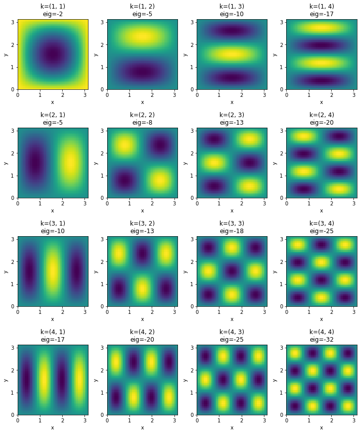
This means that our error due to truncating the span of {$\Phi_{\textbf{k}}$} at a finite number of basis fields $N$ is well defined: we can’t simulate vortices smaller than a given size.

Simulating the Fluid Dynamics

A fluid’s velocity changes over time according to physical laws. In the eigenfluid algorithm, we will simulate our fluid over time by changing the basis coefficient vector $\boldsymbol w$. By making some further observations about our choosen basis fields, and connecting them with the Navier-Stokes equations that govern fluid phenomena, we can derive a time evolution equation only in terms of $\boldsymbol w$, making its time derivative

$$ \dot w_k = \overbrace{ \boldsymbol{w}^T \boldsymbol C_k \boldsymbol w }^{\text{Advection}} + \overbrace{\nu \lambda_{k} w_{k}}^{\text{Viscosity}} + \overbrace{f_k}^{External Forces}, $$

where $\nu$ is the viscosity coefficient, and the $C_k, (k=[0…N-1])$ matrices store the precalculated advection dynamics present in the vorticity formulation of the Navier-Stokes equation. The $\textbf{f}=[f_0 \dots f_N]$ force vector is an optional external force in the base of our (vorticity) basis fields.

An Eigenfluid Simulation

Grid-based version for comparison

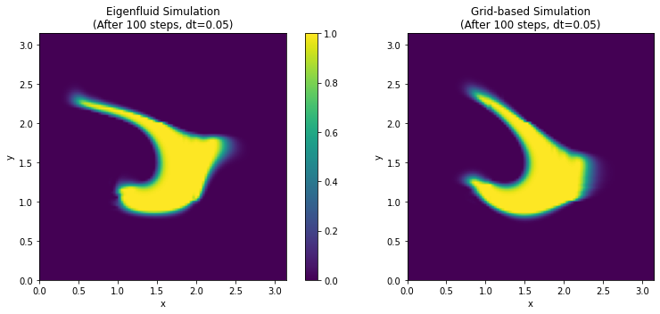
Note that even by using only $N=16$ basis fields, the eigenfluid results are comparable to a simulation on a $60\times 60$ grid. As mentioned above, the eigenfluid simulation is completely independent of the grid resolution, which was reconstructed only for the purpose of advecting the grid-based marker density. The grid-based simulation took $\approx 37$ seconds to complete, while the eigenfluid took only $\approx 19$ seconds. But most importantly, note that when simulating the eigenfluids, we were reconstructing the velocity field on a grid each time step only for advecting (or visual) purposes. Without this added reconstruction step, the simulation took only $\approx 8$ seconds.⁵

After getting an overall feel for the most important aspects of the eigenfluid simulation method, now for the fun part!

Optimization for Solution of Inverse Problems

Many real world applications require us to optimize for some parameters of a physics-based problem. A toy problem would be to optimize for some initial angle and velocity of a projectile to hit some target⁶. For a more involved example we can also think of finding the best shape for a vehicle to minimize its drag.⁷ These kinds of inverse problems have been around for quite some time in engineering applications.

In the following, we will showcase an optimization scenario, where we try to find an initial base coefficient vector $\textbf{w}^{0}$ for an eigenfluid simulation with $N=16$ basis fields, such that when simulated for $t$ time steps, the reconstructed velocity field will advect a set of initial points $\textbf{p}^0 = [p^0_0\dots p^i_0]$ to line up with target positions $\textbf{p}^{t} = [p^t_0\dots p^t_i] (i = [1, \text{number of sample points}])$. We can write this optimization problem as

$$ \arg\min_{\textbf{w}} \text{Loss}(\textbf{w}, \textbf{p}^0, \textbf{p}^t) $$

$$ = \arg\min_{\textbf{w}} \left| \mathcal{P}^{t}(\textbf{p}^0, \textbf{w}) - \textbf{p}^t\right|_2^2 $$

$$ = \arg\min_{\textbf{w}} \sum_{i}\left|\mathcal{P}^{t}(p^0_i, \textbf{w}) - p^t_i\right|_2^2, $$

where $\mathcal{P}^t(\textbf{w}, \textbf{p}) = \underbrace{\mathcal{P} \circ \mathcal{P} \dots \circ \mathcal{P}(\textbf{w}, \textbf{p})}_{t \text{ times}}$ denotes the physical simulation of base coefficients $\omega$ and points $\textbf{p}$ in the velocity field reconstructed from $\textbf{w}$. We use a simple mean-square error (or L2 norm) for measuring the error.

The main difficulty of this non-linear optimization problem lies in that we have no control over the natural flow of the fluid besides supplying an initial $\textbf{w}^0$ vector.

Making use of the differentiability of our fluid eigenfluid-solver $\mathcal{P}$, and the multivariable chain rule for deriving the gradient of the above $\mathcal{P}^t$ function composition, we can derive its gradient with respect to the initial coefficients:

$$ \frac{\partial \mathcal{P}^t(\textbf{w},\textbf{p})}{\partial \textbf{w}}. $$

And finally, we can simply iterate a gradient descent optimizer with learning rate $\mu$ to find a (good enough) solution for our above minimization problem:

$$ \textbf{w}_{\text{better}} = \textbf{w} - \mu \frac{ \partial\text{Loss}(\textbf{w}, \textbf{p}_0, \textbf{p}^t) }{ \partial \textbf{w} } $$

Results

Putting all of the above together, here are some of our current results in a visual format. The main idea is to approximate a smoke density with a given number of initial points $\textbf{p}$, and trying to approximate another target shape approximated in the same manner, with corresponding points $\textbf{p}^t$ to be reached after a predefined time $t$.

Next Steps

As mentioned in the beginning, this project is still in progress. After showing that it is feasible to use the gradients of an eigenfluid simulation for optimization, our next steps will be training Neural Network (NN) agents via these gradients to derive a generalized solution for the above shape transitions. Note that, the above results are individual optimization problems, whereas a future solution will use NNs to give a generalized solution for the set of arbitrary shape transition problems.

There are also many more interesting directions to take, among which the generalization to 3D space seems a particularly inviting next step, as all of the above methods generalize to higher dimensions in a straightforward way. We would also expect to see a significant speed-up from the point-wise reconstruction for a similar transfer problem in 3D.

Stay tuned for an update! :) Also, feel free to reach out to me with any ideas or remarks.

Sources, References & Inspirations

Eigenfluids

Tyler De Witt, Christian Lessig, and Eugene Fiume. Fluid simulation using Laplacian eigenfunctions. ACM Trans. Graph. 2012.

Qiaodong Cui, Pradeep Sen, and Theodore Kim. Scalable Laplacian Eigenfluids ACM Trans. Graph. 2018

Gradients from Physics-based Simulations

Putting deep learning in the context of physics-based simulations, and using gradients of differentiable physics solvers is spearheaded by the Thuerey Group at TUM , and our research is greatly inspired by their Physics-based Deep Learning Book .

The 2020 ICLR paper Learning to Control PDEs with Differentiable Physics served as inspiration for the problem statement of the optimization. They also released ΦFlow , an open-source simulation toolkit for optimization and machine learning applications, which we are utilizing for the implementation part.